KAFKA STREAMS CONCEPTS

INTRODUCTION RUN DEMO APP TUTORIAL: WRITE APP CONCEPTS ARCHITECTURE DEVELOPER GUIDE UPGRADE

Kafka Streams is a client library for processing and analyzing data stored in Kafka. It builds upon important stream processing concepts such as properly distinguishing between event time and processing time, windowing support, and simple yet efficient management and real-time querying of application state.

Kafka Streams has a low barrier to entry: You can quickly write and run a small-scale proof-of-concept on a single machine; and you only need to run additional instances of your application on multiple machines to scale up to high-volume production workloads. Kafka Streams transparently handles the load balancing of multiple instances of the same application by leveraging Kafka’s parallelism model.

Some highlights of Kafka Streams:

• Designed as a simple and lightweight client library, which can be easily embedded in any Java application and integrated with any existing packaging, deployment and operational tools that users have for their streaming applications.
• Has no external dependencies on systems other than Apache Kafka itself as the internal messaging layer; notably, it uses Kafka’s partitioning model to horizontally scale processing while maintaining strong ordering guarantees.
• Supports fault-tolerant local state, which enables very fast and efficient stateful operations like windowed joins and aggregations.
• Supports exactly-once processing semantics to guarantee that each record will be processed once and only once even when there is a failure on either Streams clients or Kafka brokers in the middle of processing.
• Employs one-record-at-a-time processing to achieve millisecond processing latency, and supports event-time based windowing operations with out-of-order arrival of records.
• Offers necessary stream processing primitives, along with a high-level Streams DSL and a low-level Processor API.

We first summarize the key concepts of Kafka Streams.

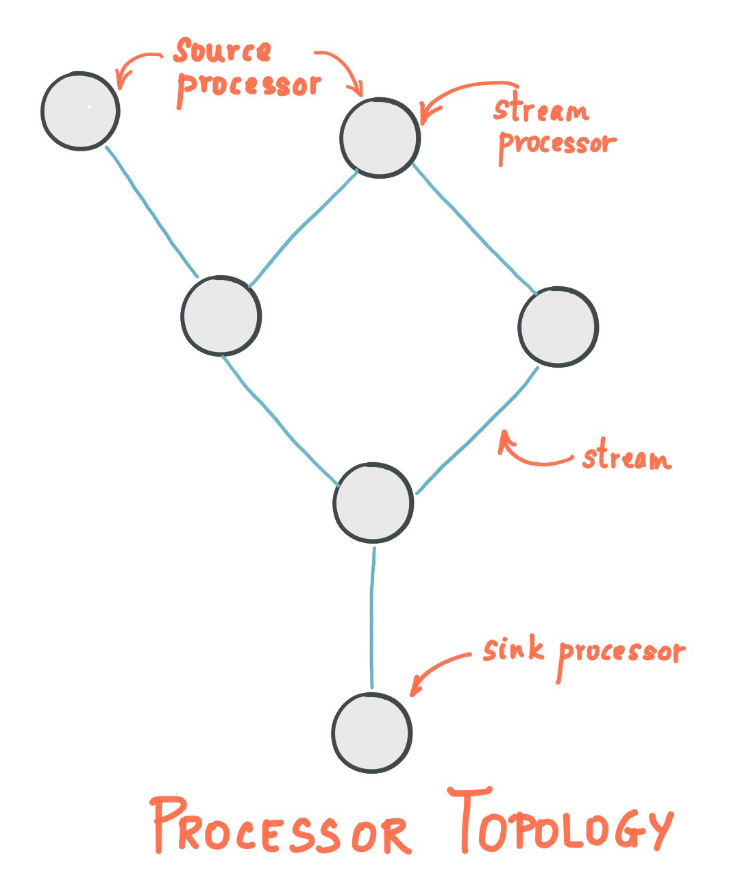
Stream Processing Topology

• A stream is the most important abstraction provided by Kafka Streams: it represents an unbounded, continuously updating data set. A stream is an ordered, replayable, and fault-tolerant sequence of immutable data records, where a data record is defined as a key-value pair.
• A stream processing application is any program that makes use of the Kafka Streams library. It defines its computational logic through one or more processor topologies, where a processor topology is a graph of stream processors (nodes) that are connected by streams (edges).
• A stream processor is a node in the processor topology; it represents a processing step to transform data in streams by receiving one input record at a time from its upstream processors in the topology, applying its operation to it, and may subsequently produce one or more output records to its downstream processors.

There are two special processors in the topology:

• Source Processor: A source processor is a special type of stream processor that does not have any upstream processors. It produces an input stream to its topology from one or multiple Kafka topics by consuming records from these topics and forwarding them to its down-stream processors.
• Sink Processor: A sink processor is a special type of stream processor that does not have down-stream processors. It sends any received records from its up-stream processors to a specified Kafka topic.

Note that in normal processor nodes other remote systems can also be accessed while processing the current record. Therefore the processed results can either be streamed back into Kafka or written to an external system.

Kafka Streams offers two ways to define the stream processing topology: the Kafka Streams DSL provides the most common data transformation operations such as map, filter, join and aggregations out of the box; the lower-level Processor API allows developers define and connect custom processors as well as to interact with state stores.

A processor topology is merely a logical abstraction for your stream processing code. At runtime, the logical topology is instantiated and replicated inside the application for parallel processing (see Stream Partitions and Tasks for details).

Time

A critical aspect in stream processing is the notion of time, and how it is modeled and integrated. For example, some operations such as windowing are defined based on time boundaries.

Common notions of time in streams are:

• Event time – The point in time when an event or data record occurred, i.e. was originally created "at the source". Example: If the event is a geo-location change reported by a GPS sensor in a car, then the associated event-time would be the time when the GPS sensor captured the location change.
• Processing time – The point in time when the event or data record happens to be processed by the stream processing application, i.e. when the record is being consumed. The processing time may be milliseconds, hours, or days etc. later than the original event time. Example: Imagine an analytics application that reads and processes the geo-location data reported from car sensors to present it to a fleet management dashboard. Here, processing-time in the analytics application might be milliseconds or seconds (e.g. for real-time pipelines based on Apache Kafka and Kafka Streams) or hours (e.g. for batch pipelines based on Apache Hadoop or Apache Spark) after event-time.
• Ingestion time – The point in time when an event or data record is stored in a topic partition by a Kafka broker. The difference to event time is that this ingestion timestamp is generated when the record is appended to the target topic by the Kafka broker, not when the record is created "at the source". The difference to processing time is that processing time is when the stream processing application processes the record. For example, if a record is never processed, there is no notion of processing time for it, but it still has an ingestion time.

The choice between event-time and ingestion-time is actually done through the configuration of Kafka (not Kafka Streams): From Kafka 0.10.x onwards, timestamps are automatically embedded into Kafka messages. Depending on Kafka’s configuration these timestamps represent event-time or ingestion-time. The respective Kafka configuration setting can be specified on the broker level or per topic. The default timestamp extractor in Kafka Streams will retrieve these embedded timestamps as-is. Hence, the effective time semantics of your application depend on the effective Kafka configuration for these embedded timestamps.

Kafka Streams assigns a timestamp to every data record via the TimestampExtractor interface. These per-record timestamps describe the progress of a stream with regards to time and are leveraged by time-dependent operations such as window operations. As a result, this time will only advance when a new record arrives at the processor. We call this data-driven time the stream time of the application to differentiate with the wall-clock time when this application is actually executing. Concrete implementations of the TimestampExtractor interface will then provide different semantics to the stream time definition. For example retrieving or computing timestamps based on the actual contents of data records such as an embedded timestamp field to provide event time semantics, and returning the current wall-clock time thereby yield processing time semantics to stream time. Developers can thus enforce different notions of time depending on their business needs.

Finally, whenever a Kafka Streams application writes records to Kafka, then it will also assign timestamps to these new records. The way the timestamps are assigned depends on the context:

• When new output records are generated via processing some input record, for example, context.forward() triggered in the process() function call, output record timestamps are inherited from input record timestamps directly.
• When new output records are generated via periodic functions such as Punctuator#punctuate(), the output record timestamp is defined as the current internal time (obtained through context.timestamp()) of the stream task.
• For aggregations, the timestamp of a result update record will be the maximum timestamp of all input records contributing to the result.

You can change the default behavior in the Processor API by assigning timestamps to output records explicitly when calling #forward().

For aggregations and joins, timestamps are computed by using the following rules.

• For joins (stream-stream, table-table) that have left and right input records, the timestamp of the output record is assigned max(left.ts, right.ts).
• For stream-table joins, the output record is assigned the timestamp from the stream record.
• For aggregations, Kafka Streams also computes the max timestamp over all records, per key, either globally (for non-windowed) or per-window.
• For stateless operations, the input record timestamp is passed through. For flatMap and siblings that emit multiple records, all output records inherit the timestamp from the corresponding input record.

Duality of Streams and Tables

When implementing stream processing use cases in practice, you typically need both streams and also databases. An example use case that is very common in practice is an e-commerce application that enriches an incoming stream of customer transactions with the latest customer information from a database table. In other words, streams are everywhere, but databases are everywhere, too.

Any stream processing technology must therefore provide first-class support for streams and tables. Kafka’s Streams API provides such functionality through its core abstractions for streams and tables, which we will talk about in a minute. Now, an interesting observation is that there is actually a close relationship between streams and tables, the so-called stream-table duality. And Kafka exploits this duality in many ways: for example, to make your applications elastic, to support fault-tolerant stateful processing, or to run interactive queries against your application’s latest processing results. And, beyond its internal usage, the Kafka Streams API also allows developers to exploit this duality in their own applications.

Before we discuss concepts such as aggregations in Kafka Streams, we must first introduce tables in more detail, and talk about the aforementioned stream-table duality. Essentially, this duality means that a stream can be viewed as a table, and a table can be viewed as a stream. Kafka’s log compaction feature, for example, exploits this duality.

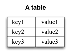
A simple form of a table is a collection of key-value pairs, also called a map or associative array. Such a table may look as follows:

The stream-table duality describes the close relationship between streams and tables.

• Stream as Table: A stream can be considered a changelog of a table, where each data record in the stream captures a state change of the table. A stream is thus a table in disguise, and it can be easily turned into a "real" table by replaying the changelog from beginning to end to reconstruct the table. Similarly, in a more general analogy, aggregating data records in a stream – such as computing the total number of pageviews by user from a stream of pageview events – will return a table (here with the key and the value being the user and its corresponding pageview count, respectively).
• Table as Stream: A table can be considered a snapshot, at a point in time, of the latest value for each key in a stream (a stream’s data records are key-value pairs). A table is thus a stream in disguise, and it can be easily turned into a "real" stream by iterating over each key-value entry in the table.

Let’s illustrate this with an example. Imagine a table that tracks the total number of pageviews by user (first column of diagram below). Over time, whenever a new pageview event is processed, the state of the table is updated accordingly. Here, the state changes between different points in time – and different revisions of the table – can be represented as a changelog stream (second column).

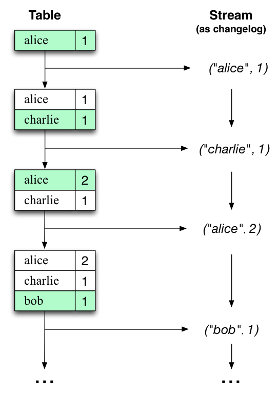
Interestingly, because of the stream-table duality, the same stream can be used to reconstruct the original table (third column):

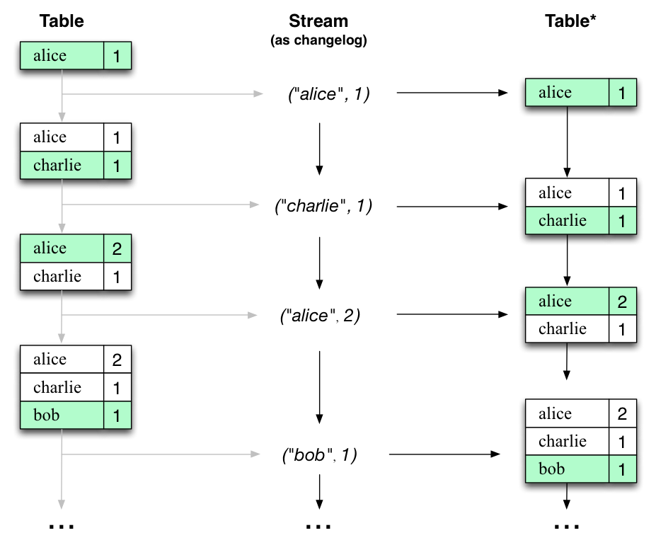
The same mechanism is used, for example, to replicate databases via change data capture (CDC) and, within Kafka Streams, to replicate its so-called state stores across machines for fault-tolerance. The stream-table duality is such an important concept that Kafka Streams models it explicitly via the KStream, KTable, and GlobalKTable interfaces.

Aggregations

An aggregation operation takes one input stream or table, and yields a new table by combining multiple input records into a single output record. Examples of aggregations are computing counts or sum.

In the Kafka Streams DSL, an input stream of an aggregation can be a KStream or a KTable, but the output stream will always be a KTable. This allows Kafka Streams to update an aggregate value upon the out-of-order arrival of further records after the value was produced and emitted. When such out-of-order arrival happens, the aggregating KStream or KTable emits a new aggregate value. Because the output is a KTable, the new value is considered to overwrite the old value with the same key in subsequent processing steps.

Windowing

Windowing lets you control how to group records that have the same key for stateful operations such as aggregations or joins into so-called windows. Windows are tracked per record key.

Windowing operations are available in the Kafka Streams DSL. When working with windows, you can specify a grace period for the window. This grace period controls how long Kafka Streams will wait for out-of-order data records for a given window. If a record arrives after the grace period of a window has passed, the record is discarded and will not be processed in that window. Specifically, a record is discarded if its timestamp dictates it belongs to a window, but the current stream time is greater than the end of the window plus the grace period.

Out-of-order records are always possible in the real world and should be properly accounted for in your applications. It depends on the effective time semantics how out-of-order records are handled. In the case of processing-time, the semantics are "when the record is being processed", which means that the notion of out-of-order records is not applicable as, by definition, no record can be out-of-order. Hence, out-of-order records can only be considered as such for event-time. In both cases, Kafka Streams is able to properly handle out-of-order records.

States

Some stream processing applications don’t require state, which means the processing of a message is independent from the processing of all other messages. However, being able to maintain state opens up many possibilities for sophisticated stream processing applications: you can join input streams, or group and aggregate data records. Many such stateful operators are provided by the Kafka Streams DSL.

Kafka Streams provides so-called state stores, which can be used by stream processing applications to store and query data. This is an important capability when implementing stateful operations. Every task in Kafka Streams embeds one or more state stores that can be accessed via APIs to store and query data required for processing. These state stores can either be a persistent key-value store, an in-memory hashmap, or another convenient data structure. Kafka Streams offers fault-tolerance and automatic recovery for local state stores.

Kafka Streams allows direct read-only queries of the state stores by methods, threads, processes or applications external to the stream processing application that created the state stores. This is provided through a feature called Interactive Queries. All stores are named and Interactive Queries exposes only the read operations of the underlying implementation.

PROCESSING GUARANTEES

In stream processing, one of the most frequently asked question is "does my stream processing system guarantee that each record is processed once and only once, even if some failures are encountered in the middle of processing?" Failing to guarantee exactly-once stream processing is a deal-breaker for many applications that cannot tolerate any data-loss or data duplicates, and in that case a batch-oriented framework is usually used in addition to the stream processing pipeline, known as the Lambda Architecture. Prior to 0.11.0.0, Kafka only provides at-least-once delivery guarantees and hence any stream processing systems that leverage it as the backend storage could not guarantee end-to-end exactly-once semantics. In fact, even for those stream processing systems that claim to support exactly-once processing, as long as they are reading from / writing to Kafka as the source / sink, their applications cannot actually guarantee that no duplicates will be generated throughout the pipeline.
Since the 0.11.0.0 release, Kafka has added support to allow its producers to send messages to different topic partitions in a transactional and idempotent manner, and Kafka Streams has hence added the end-to-end exactly-once processing semantics by leveraging these features. More specifically, it guarantees that for any record read from the source Kafka topics, its processing results will be reflected exactly once in the output Kafka topic as well as in the state stores for stateful operations. Note the key difference between Kafka Streams end-to-end exactly-once guarantee with other stream processing frameworks’ claimed guarantees is that Kafka Streams tightly integrates with the underlying Kafka storage system and ensure that commits on the input topic offsets, updates on the state stores, and writes to the output topics will be completed atomically instead of treating Kafka as an external system that may have side-effects. For more information on how this is done inside Kafka Streams, see KIP-129.
As of the 2.6.0 release, Kafka Streams supports an improved implementation of exactly-once processing, named "exactly-once v2", which requires broker version 2.5.0 or newer. This implementation is more efficient, because it reduces client and broker resource utilization, like client threads and used network connections, and it enables higher throughput and improved scalability. As of the 3.0.0 release, the first version of exactly-once has been deprecated. Users are encouraged to use exactly-once v2 for exactly-once processing from now on, and prepare by upgrading their brokers if necessary. For more information on how this is done inside the brokers and Kafka Streams, see KIP-447.
To enable exactly-once semantics when running Kafka Streams applications, set the processing.guarantee config value (default value is at_least_once) to StreamsConfig.EXACTLY_ONCE_V2 (requires brokers version 2.5 or newer). For more information, see the Kafka Streams Configs section.

Out-of-Order Handling

Besides the guarantee that each record will be processed exactly-once, another issue that many stream processing application will face is how to handle out-of-order data that may impact their business logic. In Kafka Streams, there are two causes that could potentially result in out-of-order data arrivals with respect to their timestamps:

• Within a topic-partition, a record’s timestamp may not be monotonically increasing along with their offsets. Since Kafka Streams will always try to process records within a topic-partition to follow the offset order, it can cause records with larger timestamps (but smaller offsets) to be processed earlier than records with smaller timestamps (but larger offsets) in the same topic-partition.
• Within a stream task that may be processing multiple topic-partitions, if users configure the application to not wait for all partitions to contain some buffered data and pick from the partition with the smallest timestamp to process the next record, then later on when some records are fetched for other topic-partitions, their timestamps may be smaller than those processed records fetched from another topic-partition.

For stateless operations, out-of-order data will not impact processing logic since only one record is considered at a time, without looking into the history of past processed records; for stateful operations such as aggregations and joins, however, out-of-order data could cause the processing logic to be incorrect. If users want to handle such out-of-order data, generally they need to allow their applications to wait for longer time while bookkeeping their states during the wait time, i.e. making trade-off decisions between latency, cost, and correctness. In Kafka Streams specifically, users can configure their window operators for windowed aggregations to achieve such trade-offs (details can be found in Developer Guide). As for Joins, users have to be aware that some of the out-of-order data cannot be handled by increasing on latency and cost in Streams yet:

• For Stream-Stream joins, all three types (inner, outer, left) handle out-of-order records correctly, but the resulted stream may contain unnecessary leftRecord-null for left joins, and leftRecord-null or null-rightRecord for outer joins.
• For Stream-Table joins, out-of-order records are not handled (i.e., Streams applications don’t check for out-of-order records and just process all records in offset order), and hence it may produce unpredictable results.
• For Table-Table joins, out-of-order records are not handled (i.e., Streams applications don’t check for out-of-order records and just process all records in offset order). However, the join result is a changelog stream and hence will be eventually consistent.

Views: 123