KAFKA STREAMS ARCHITECTURE

Kafka Streams simplifies application development by building on the Kafka producer and consumer libraries and leveraging the native capabilities of Kafka to offer data parallelism, distributed coordination, fault tolerance, and operational simplicity. In this section, we describe how Kafka Streams works underneath the covers.

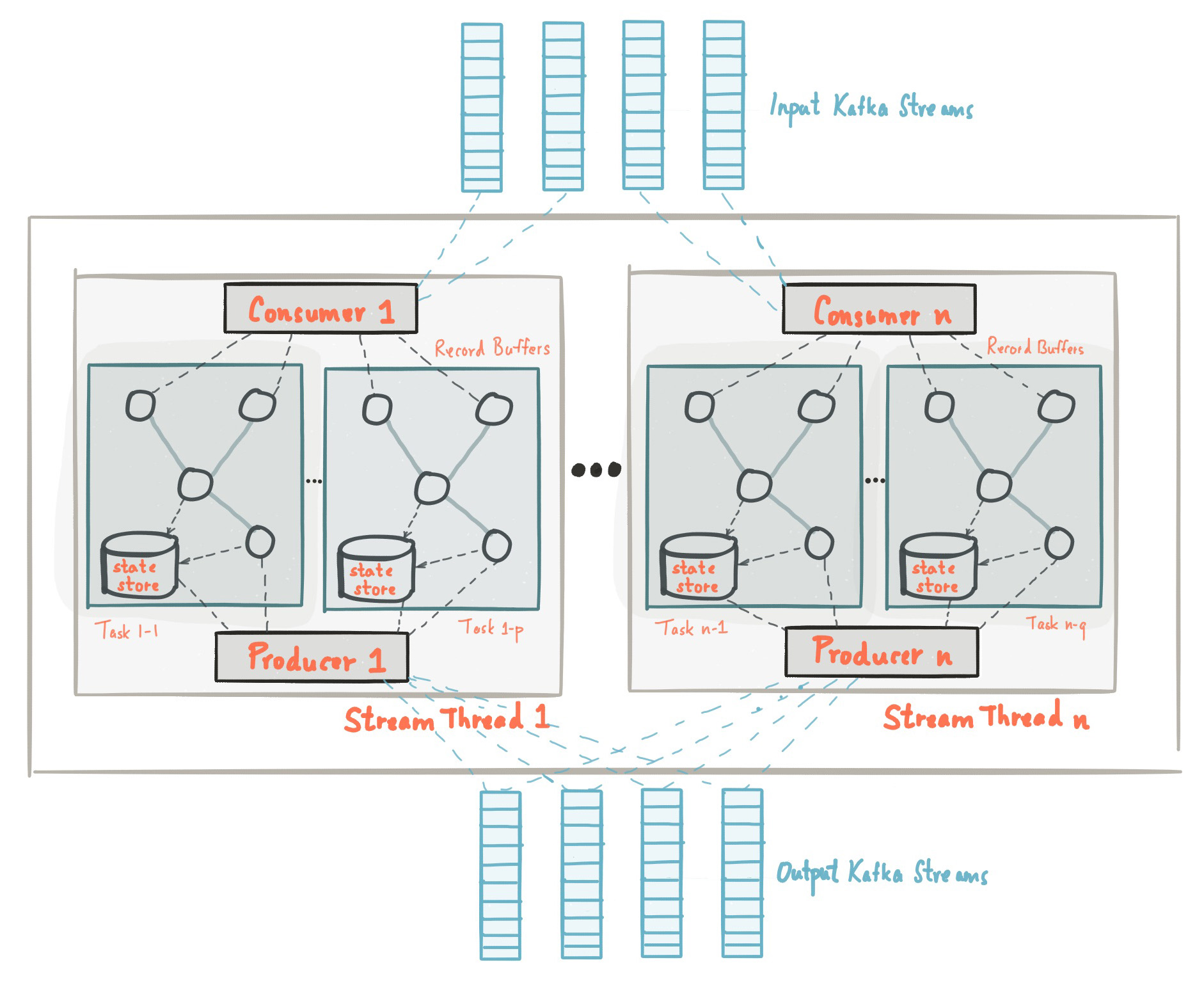
The picture below shows the anatomy of an application that uses the Kafka Streams library. Let's walk through some details.

img

Stream Partitions and Tasks

The messaging layer of Kafka partitions data for storing and transporting it. Kafka Streams partitions data for processing it. In both cases, this partitioning is what enables data locality, elasticity, scalability, high performance, and fault tolerance. Kafka Streams uses the concepts of partitions and tasks as logical units of its parallelism model based on Kafka topic partitions. There are close links between Kafka Streams and Kafka in the context of parallelism:

  • Each stream partition is a totally ordered sequence of data records and maps to a Kafka topic partition.
  • A data record in the stream maps to a Kafka message from that topic.
  • The keys of data records determine the partitioning of data in both Kafka and Kafka Streams, i.e., how data is routed to specific partitions within topics.

An application's processor topology is scaled by breaking it into multiple tasks. More specifically, Kafka Streams creates a fixed number of tasks based on the input stream partitions for the application, with each task assigned a list of partitions from the input streams (i.e., Kafka topics). The assignment of partitions to tasks never changes so that each task is a fixed unit of parallelism of the application. Tasks can then instantiate their own processor topology based on the assigned partitions; they also maintain a buffer for each of its assigned partitions and process messages one-at-a-time from these record buffers. As a result stream tasks can be processed independently and in parallel without manual intervention.

Slightly simplified, the maximum parallelism at which your application may run is bounded by the maximum number of stream tasks, which itself is determined by maximum number of partitions of the input topic(s) the application is reading from. For example, if your input topic has 5 partitions, then you can run up to 5 applications instances. These instances will collaboratively process the topic’s data. If you run a larger number of app instances than partitions of the input topic, the “excess” app instances will launch but remain idle; however, if one of the busy instances goes down, one of the idle instances will resume the former’s work.

It is important to understand that Kafka Streams is not a resource manager, but a library that "runs" anywhere its stream processing application runs. Multiple instances of the application are executed either on the same machine, or spread across multiple machines and tasks can be distributed automatically by the library to those running application instances. The assignment of partitions to tasks never changes; if an application instance fails, all its assigned tasks will be automatically restarted on other instances and continue to consume from the same stream partitions.

NOTE: Topic partitions are assigned to tasks, and tasks are assigned to all threads over all instances, in a best-effort attempt to trade off load-balancing and stickiness of stateful tasks. For this assignment, Kafka Streams uses the StreamsPartitionAssignor class and doesn't let you change to a different assignor. If you try to use a different assignor, Kafka Streams ignores it.

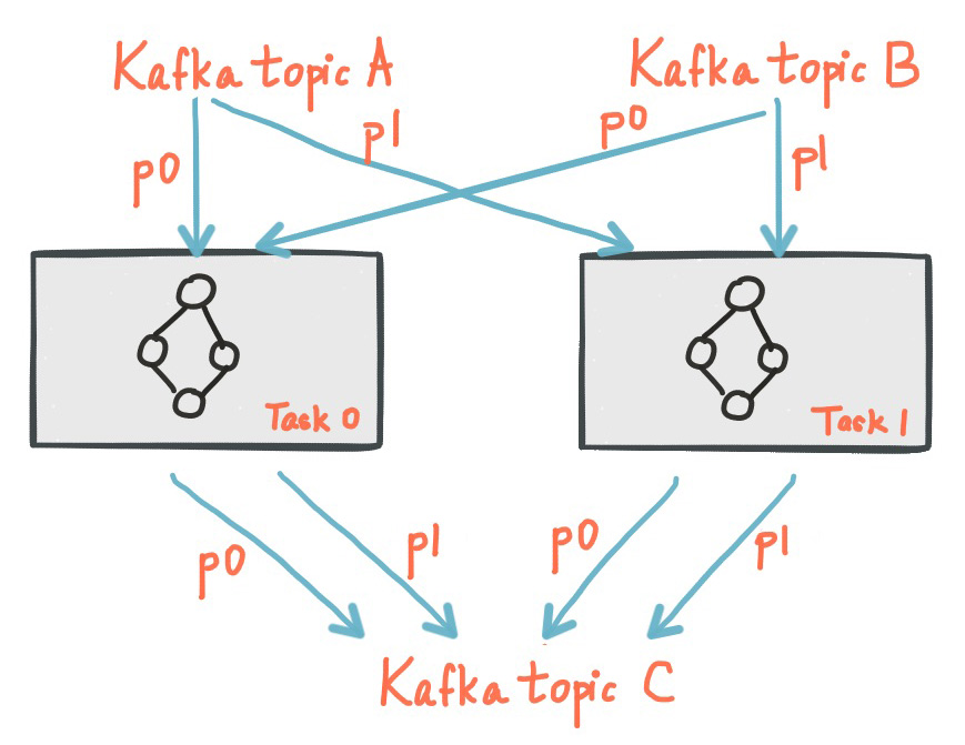
The following diagram shows two tasks each assigned with one partition of the input streams.

img

Threading Model

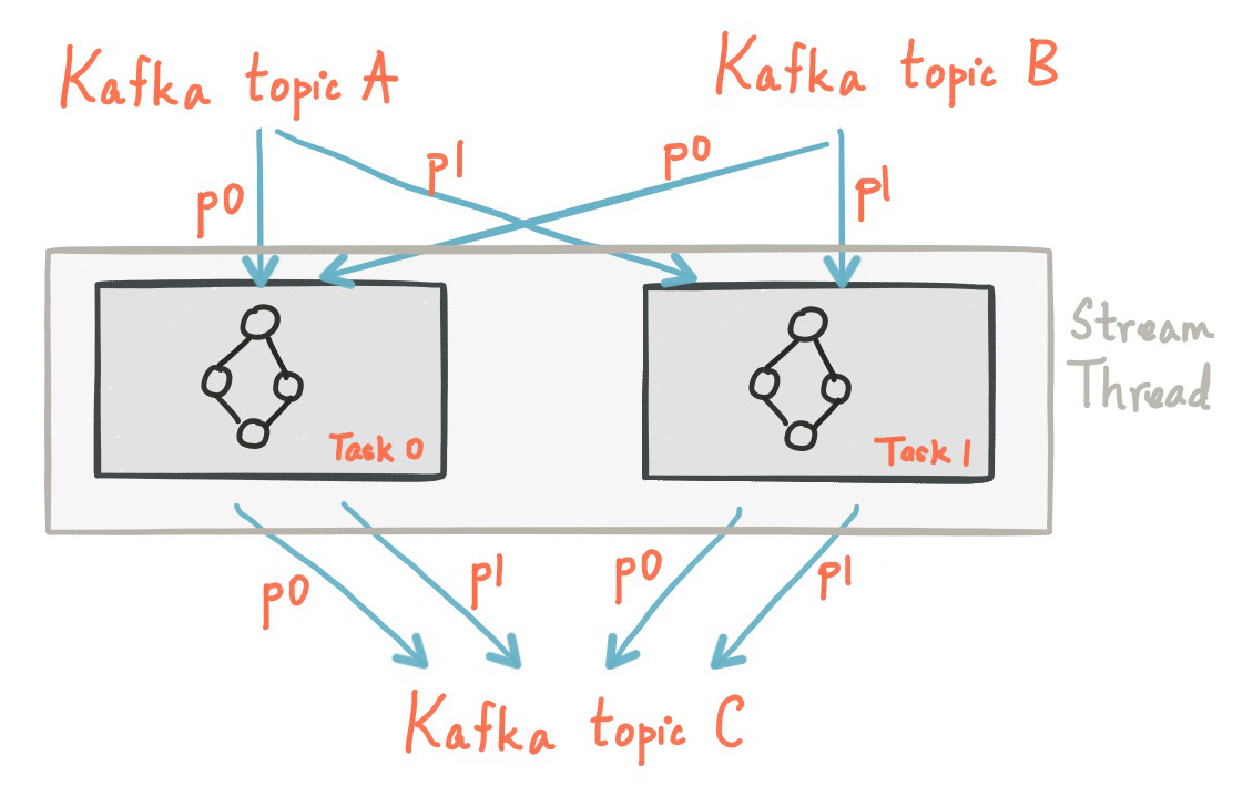
Kafka Streams allows the user to configure the number of threads that the library can use to parallelize processing within an application instance. Each thread can execute one or more tasks with their processor topologies independently. For example, the following diagram shows one stream thread running two stream tasks.

img

Starting more stream threads or more instances of the application merely amounts to replicating the topology and having it process a different subset of Kafka partitions, effectively parallelizing processing. It is worth noting that there is no shared state amongst the threads, so no inter-thread coordination is necessary. This makes it very simple to run topologies in parallel across the application instances and threads. The assignment of Kafka topic partitions amongst the various stream threads is transparently handled by Kafka Streams leveraging Kafka's coordination functionality.

As we described above, scaling your stream processing application with Kafka Streams is easy: you merely need to start additional instances of your application, and Kafka Streams takes care of distributing partitions amongst tasks that run in the application instances. You can start as many threads of the application as there are input Kafka topic partitions so that, across all running instances of an application, every thread (or rather, the tasks it runs) has at least one input partition to process.

As of Kafka 2.8 you can scale stream threads much in the same way you can scale your Kafka Stream clients. Simply add or remove stream threads and Kafka Streams will take care of redistributing the partitions. You may also add threads to replace stream threads that have died removing the need to restart clients to recover the number of thread running.

Local State Stores

Kafka Streams provides so-called state stores, which can be used by stream processing applications to store and query data, which is an important capability when implementing stateful operations. The Kafka Streams DSL, for example, automatically creates and manages such state stores when you are calling stateful operators such as join() or aggregate(), or when you are windowing a stream.

Every stream task in a Kafka Streams application may embed one or more local state stores that can be accessed via APIs to store and query data required for processing. Kafka Streams offers fault-tolerance and automatic recovery for such local state stores.

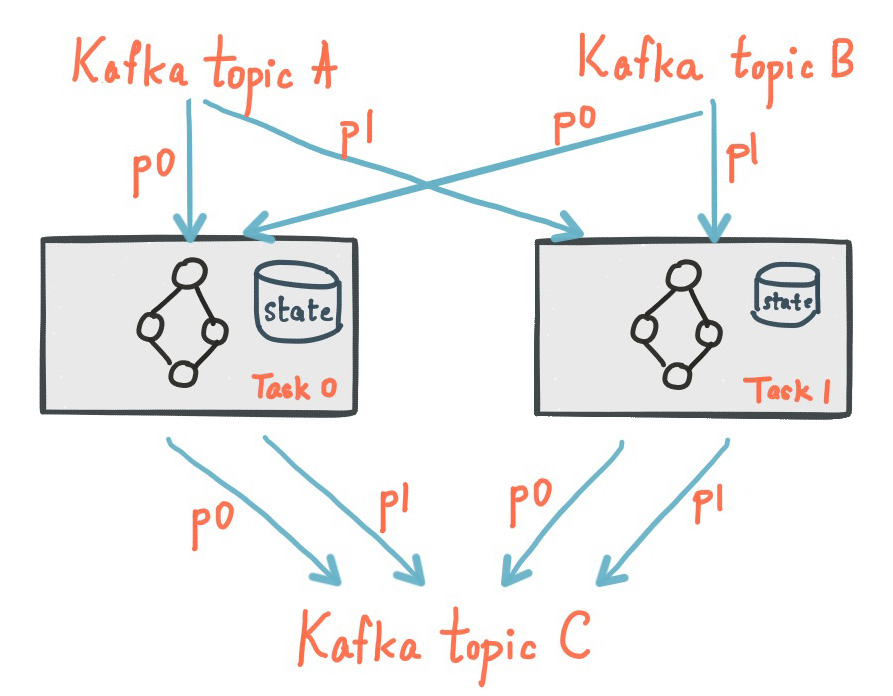
The following diagram shows two stream tasks with their dedicated local state stores.

img

Fault Tolerance

Kafka Streams builds on fault-tolerance capabilities integrated natively within Kafka. Kafka partitions are highly available and replicated; so when stream data is persisted to Kafka it is available even if the application fails and needs to re-process it. Tasks in Kafka Streams leverage the fault-tolerance capability offered by the Kafka consumer client to handle failures. If a task runs on a machine that fails, Kafka Streams automatically restarts the task in one of the remaining running instances of the application.

In addition, Kafka Streams makes sure that the local state stores are robust to failures, too. For each state store, it maintains a replicated changelog Kafka topic in which it tracks any state updates. These changelog topics are partitioned as well so that each local state store instance, and hence the task accessing the store, has its own dedicated changelog topic partition. Log compaction is enabled on the changelog topics so that old data can be purged safely to prevent the topics from growing indefinitely. If tasks run on a machine that fails and are restarted on another machine, Kafka Streams guarantees to restore their associated state stores to the content before the failure by replaying the corresponding changelog topics prior to resuming the processing on the newly started tasks. As a result, failure handling is completely transparent to the end user.

Note that the cost of task (re)initialization typically depends primarily on the time for restoring the state by replaying the state stores' associated changelog topics. To minimize this restoration time, users can configure their applications to have standby replicas of local states (i.e. fully replicated copies of the state). When a task migration happens, Kafka Streams will assign a task to an application instance where such a standby replica already exists in order to minimize the task (re)initialization cost. See num.standby.replicas in the Kafka Streams Configs section. Starting in 2.6, Kafka Streams will guarantee that a task is only ever assigned to an instance with a fully caught-up local copy of the state, if such an instance exists. Standby tasks will increase the likelihood that a caught-up instance exists in the case of a failure.

Views: 201

KAFKA STREAMS CONCEPTS

INTRODUCTION RUN DEMO APP TUTORIAL: WRITE APP CONCEPTS ARCHITECTURE DEVELOPER GUIDE UPGRADE

Kafka Streams is a client library for processing and analyzing data stored in Kafka. It builds upon important stream processing concepts such as properly distinguishing between event time and processing time, windowing support, and simple yet efficient management and real-time querying of application state.

Kafka Streams has a low barrier to entry: You can quickly write and run a small-scale proof-of-concept on a single machine; and you only need to run additional instances of your application on multiple machines to scale up to high-volume production workloads. Kafka Streams transparently handles the load balancing of multiple instances of the same application by leveraging Kafka's parallelism model.

Some highlights of Kafka Streams:

  • Designed as a simple and lightweight client library, which can be easily embedded in any Java application and integrated with any existing packaging, deployment and operational tools that users have for their streaming applications.
  • Has no external dependencies on systems other than Apache Kafka itself as the internal messaging layer; notably, it uses Kafka's partitioning model to horizontally scale processing while maintaining strong ordering guarantees.
  • Supports fault-tolerant local state, which enables very fast and efficient stateful operations like windowed joins and aggregations.
  • Supports exactly-once processing semantics to guarantee that each record will be processed once and only once even when there is a failure on either Streams clients or Kafka brokers in the middle of processing.
  • Employs one-record-at-a-time processing to achieve millisecond processing latency, and supports event-time based windowing operations with out-of-order arrival of records.
  • Offers necessary stream processing primitives, along with a high-level Streams DSL and a low-level Processor API.

We first summarize the key concepts of Kafka Streams.

Stream Processing Topology

  • A stream is the most important abstraction provided by Kafka Streams: it represents an unbounded, continuously updating data set. A stream is an ordered, replayable, and fault-tolerant sequence of immutable data records, where a data record is defined as a key-value pair.
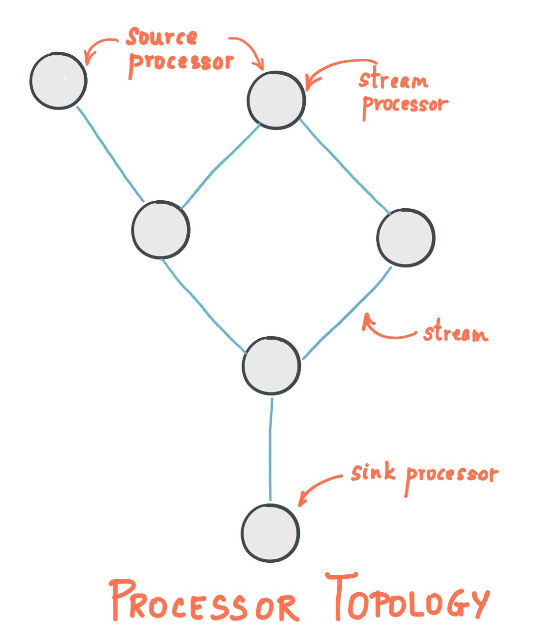
  • A stream processing application is any program that makes use of the Kafka Streams library. It defines its computational logic through one or more processor topologies, where a processor topology is a graph of stream processors (nodes) that are connected by streams (edges).
  • A stream processor is a node in the processor topology; it represents a processing step to transform data in streams by receiving one input record at a time from its upstream processors in the topology, applying its operation to it, and may subsequently produce one or more output records to its downstream processors.

There are two special processors in the topology:

  • Source Processor: A source processor is a special type of stream processor that does not have any upstream processors. It produces an input stream to its topology from one or multiple Kafka topics by consuming records from these topics and forwarding them to its down-stream processors.
  • Sink Processor: A sink processor is a special type of stream processor that does not have down-stream processors. It sends any received records from its up-stream processors to a specified Kafka topic.

Note that in normal processor nodes other remote systems can also be accessed while processing the current record. Therefore the processed results can either be streamed back into Kafka or written to an external system.

img

Kafka Streams offers two ways to define the stream processing topology: the Kafka Streams DSL provides the most common data transformation operations such as map, filter, join and aggregations out of the box; the lower-level Processor API allows developers define and connect custom processors as well as to interact with state stores.

A processor topology is merely a logical abstraction for your stream processing code. At runtime, the logical topology is instantiated and replicated inside the application for parallel processing (see Stream Partitions and Tasks for details).

Time

A critical aspect in stream processing is the notion of time, and how it is modeled and integrated. For example, some operations such as windowing are defined based on time boundaries.

Common notions of time in streams are:

  • Event time - The point in time when an event or data record occurred, i.e. was originally created "at the source". Example: If the event is a geo-location change reported by a GPS sensor in a car, then the associated event-time would be the time when the GPS sensor captured the location change.
  • Processing time - The point in time when the event or data record happens to be processed by the stream processing application, i.e. when the record is being consumed. The processing time may be milliseconds, hours, or days etc. later than the original event time. Example: Imagine an analytics application that reads and processes the geo-location data reported from car sensors to present it to a fleet management dashboard. Here, processing-time in the analytics application might be milliseconds or seconds (e.g. for real-time pipelines based on Apache Kafka and Kafka Streams) or hours (e.g. for batch pipelines based on Apache Hadoop or Apache Spark) after event-time.
  • Ingestion time - The point in time when an event or data record is stored in a topic partition by a Kafka broker. The difference to event time is that this ingestion timestamp is generated when the record is appended to the target topic by the Kafka broker, not when the record is created "at the source". The difference to processing time is that processing time is when the stream processing application processes the record. For example, if a record is never processed, there is no notion of processing time for it, but it still has an ingestion time.

The choice between event-time and ingestion-time is actually done through the configuration of Kafka (not Kafka Streams): From Kafka 0.10.x onwards, timestamps are automatically embedded into Kafka messages. Depending on Kafka's configuration these timestamps represent event-time or ingestion-time. The respective Kafka configuration setting can be specified on the broker level or per topic. The default timestamp extractor in Kafka Streams will retrieve these embedded timestamps as-is. Hence, the effective time semantics of your application depend on the effective Kafka configuration for these embedded timestamps.

Kafka Streams assigns a timestamp to every data record via the TimestampExtractor interface. These per-record timestamps describe the progress of a stream with regards to time and are leveraged by time-dependent operations such as window operations. As a result, this time will only advance when a new record arrives at the processor. We call this data-driven time the stream time of the application to differentiate with the wall-clock time when this application is actually executing. Concrete implementations of the TimestampExtractor interface will then provide different semantics to the stream time definition. For example retrieving or computing timestamps based on the actual contents of data records such as an embedded timestamp field to provide event time semantics, and returning the current wall-clock time thereby yield processing time semantics to stream time. Developers can thus enforce different notions of time depending on their business needs.

Finally, whenever a Kafka Streams application writes records to Kafka, then it will also assign timestamps to these new records. The way the timestamps are assigned depends on the context:

  • When new output records are generated via processing some input record, for example, context.forward() triggered in the process() function call, output record timestamps are inherited from input record timestamps directly.
  • When new output records are generated via periodic functions such as Punctuator#punctuate(), the output record timestamp is defined as the current internal time (obtained through context.timestamp()) of the stream task.
  • For aggregations, the timestamp of a result update record will be the maximum timestamp of all input records contributing to the result.

You can change the default behavior in the Processor API by assigning timestamps to output records explicitly when calling #forward().

For aggregations and joins, timestamps are computed by using the following rules.

  • For joins (stream-stream, table-table) that have left and right input records, the timestamp of the output record is assigned max(left.ts, right.ts).
  • For stream-table joins, the output record is assigned the timestamp from the stream record.
  • For aggregations, Kafka Streams also computes the max timestamp over all records, per key, either globally (for non-windowed) or per-window.
  • For stateless operations, the input record timestamp is passed through. For flatMap and siblings that emit multiple records, all output records inherit the timestamp from the corresponding input record.

Duality of Streams and Tables

When implementing stream processing use cases in practice, you typically need both streams and also databases. An example use case that is very common in practice is an e-commerce application that enriches an incoming stream of customer transactions with the latest customer information from a database table. In other words, streams are everywhere, but databases are everywhere, too.

Any stream processing technology must therefore provide first-class support for streams and tables. Kafka's Streams API provides such functionality through its core abstractions for streams and tables, which we will talk about in a minute. Now, an interesting observation is that there is actually a close relationship between streams and tables, the so-called stream-table duality. And Kafka exploits this duality in many ways: for example, to make your applications elastic, to support fault-tolerant stateful processing, or to run interactive queries against your application's latest processing results. And, beyond its internal usage, the Kafka Streams API also allows developers to exploit this duality in their own applications.

Before we discuss concepts such as aggregations in Kafka Streams, we must first introduce tables in more detail, and talk about the aforementioned stream-table duality. Essentially, this duality means that a stream can be viewed as a table, and a table can be viewed as a stream. Kafka's log compaction feature, for example, exploits this duality.

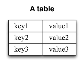
A simple form of a table is a collection of key-value pairs, also called a map or associative array. Such a table may look as follows:

img

The stream-table duality describes the close relationship between streams and tables.

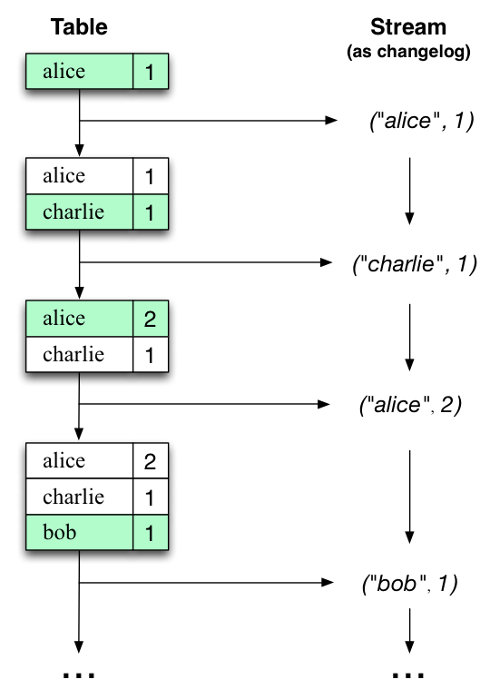
  • Stream as Table: A stream can be considered a changelog of a table, where each data record in the stream captures a state change of the table. A stream is thus a table in disguise, and it can be easily turned into a "real" table by replaying the changelog from beginning to end to reconstruct the table. Similarly, in a more general analogy, aggregating data records in a stream - such as computing the total number of pageviews by user from a stream of pageview events - will return a table (here with the key and the value being the user and its corresponding pageview count, respectively).
  • Table as Stream: A table can be considered a snapshot, at a point in time, of the latest value for each key in a stream (a stream's data records are key-value pairs). A table is thus a stream in disguise, and it can be easily turned into a "real" stream by iterating over each key-value entry in the table.

Let's illustrate this with an example. Imagine a table that tracks the total number of pageviews by user (first column of diagram below). Over time, whenever a new pageview event is processed, the state of the table is updated accordingly. Here, the state changes between different points in time - and different revisions of the table - can be represented as a changelog stream (second column).

img

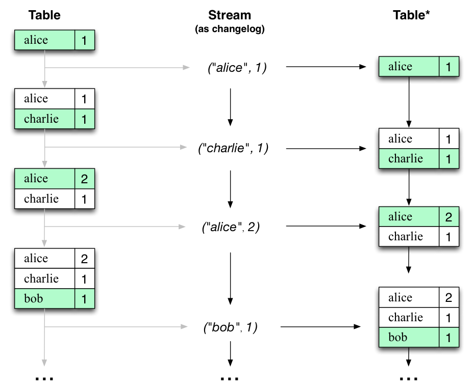
Interestingly, because of the stream-table duality, the same stream can be used to reconstruct the original table (third column):

img

The same mechanism is used, for example, to replicate databases via change data capture (CDC) and, within Kafka Streams, to replicate its so-called state stores across machines for fault-tolerance. The stream-table duality is such an important concept that Kafka Streams models it explicitly via the KStream, KTable, and GlobalKTable interfaces.

Aggregations

An aggregation operation takes one input stream or table, and yields a new table by combining multiple input records into a single output record. Examples of aggregations are computing counts or sum.

In the Kafka Streams DSL, an input stream of an aggregation can be a KStream or a KTable, but the output stream will always be a KTable. This allows Kafka Streams to update an aggregate value upon the out-of-order arrival of further records after the value was produced and emitted. When such out-of-order arrival happens, the aggregating KStream or KTable emits a new aggregate value. Because the output is a KTable, the new value is considered to overwrite the old value with the same key in subsequent processing steps.

Windowing

Windowing lets you control how to group records that have the same key for stateful operations such as aggregations or joins into so-called windows. Windows are tracked per record key.

Windowing operations are available in the Kafka Streams DSL. When working with windows, you can specify a grace period for the window. This grace period controls how long Kafka Streams will wait for out-of-order data records for a given window. If a record arrives after the grace period of a window has passed, the record is discarded and will not be processed in that window. Specifically, a record is discarded if its timestamp dictates it belongs to a window, but the current stream time is greater than the end of the window plus the grace period.

Out-of-order records are always possible in the real world and should be properly accounted for in your applications. It depends on the effective time semantics how out-of-order records are handled. In the case of processing-time, the semantics are "when the record is being processed", which means that the notion of out-of-order records is not applicable as, by definition, no record can be out-of-order. Hence, out-of-order records can only be considered as such for event-time. In both cases, Kafka Streams is able to properly handle out-of-order records.

States

Some stream processing applications don't require state, which means the processing of a message is independent from the processing of all other messages. However, being able to maintain state opens up many possibilities for sophisticated stream processing applications: you can join input streams, or group and aggregate data records. Many such stateful operators are provided by the Kafka Streams DSL.

Kafka Streams provides so-called state stores, which can be used by stream processing applications to store and query data. This is an important capability when implementing stateful operations. Every task in Kafka Streams embeds one or more state stores that can be accessed via APIs to store and query data required for processing. These state stores can either be a persistent key-value store, an in-memory hashmap, or another convenient data structure. Kafka Streams offers fault-tolerance and automatic recovery for local state stores.

Kafka Streams allows direct read-only queries of the state stores by methods, threads, processes or applications external to the stream processing application that created the state stores. This is provided through a feature called Interactive Queries. All stores are named and Interactive Queries exposes only the read operations of the underlying implementation.

PROCESSING GUARANTEES

In stream processing, one of the most frequently asked question is "does my stream processing system guarantee that each record is processed once and only once, even if some failures are encountered in the middle of processing?" Failing to guarantee exactly-once stream processing is a deal-breaker for many applications that cannot tolerate any data-loss or data duplicates, and in that case a batch-oriented framework is usually used in addition to the stream processing pipeline, known as the Lambda Architecture. Prior to 0.11.0.0, Kafka only provides at-least-once delivery guarantees and hence any stream processing systems that leverage it as the backend storage could not guarantee end-to-end exactly-once semantics. In fact, even for those stream processing systems that claim to support exactly-once processing, as long as they are reading from / writing to Kafka as the source / sink, their applications cannot actually guarantee that no duplicates will be generated throughout the pipeline.
Since the 0.11.0.0 release, Kafka has added support to allow its producers to send messages to different topic partitions in a transactional and idempotent manner, and Kafka Streams has hence added the end-to-end exactly-once processing semantics by leveraging these features. More specifically, it guarantees that for any record read from the source Kafka topics, its processing results will be reflected exactly once in the output Kafka topic as well as in the state stores for stateful operations. Note the key difference between Kafka Streams end-to-end exactly-once guarantee with other stream processing frameworks' claimed guarantees is that Kafka Streams tightly integrates with the underlying Kafka storage system and ensure that commits on the input topic offsets, updates on the state stores, and writes to the output topics will be completed atomically instead of treating Kafka as an external system that may have side-effects. For more information on how this is done inside Kafka Streams, see KIP-129.
As of the 2.6.0 release, Kafka Streams supports an improved implementation of exactly-once processing, named "exactly-once v2", which requires broker version 2.5.0 or newer. This implementation is more efficient, because it reduces client and broker resource utilization, like client threads and used network connections, and it enables higher throughput and improved scalability. As of the 3.0.0 release, the first version of exactly-once has been deprecated. Users are encouraged to use exactly-once v2 for exactly-once processing from now on, and prepare by upgrading their brokers if necessary. For more information on how this is done inside the brokers and Kafka Streams, see KIP-447.
To enable exactly-once semantics when running Kafka Streams applications, set the processing.guarantee config value (default value is at_least_once) to StreamsConfig.EXACTLY_ONCE_V2 (requires brokers version 2.5 or newer). For more information, see the Kafka Streams Configs section.

Out-of-Order Handling

Besides the guarantee that each record will be processed exactly-once, another issue that many stream processing application will face is how to handle out-of-order data that may impact their business logic. In Kafka Streams, there are two causes that could potentially result in out-of-order data arrivals with respect to their timestamps:

  • Within a topic-partition, a record's timestamp may not be monotonically increasing along with their offsets. Since Kafka Streams will always try to process records within a topic-partition to follow the offset order, it can cause records with larger timestamps (but smaller offsets) to be processed earlier than records with smaller timestamps (but larger offsets) in the same topic-partition.
  • Within a stream task that may be processing multiple topic-partitions, if users configure the application to not wait for all partitions to contain some buffered data and pick from the partition with the smallest timestamp to process the next record, then later on when some records are fetched for other topic-partitions, their timestamps may be smaller than those processed records fetched from another topic-partition.

For stateless operations, out-of-order data will not impact processing logic since only one record is considered at a time, without looking into the history of past processed records; for stateful operations such as aggregations and joins, however, out-of-order data could cause the processing logic to be incorrect. If users want to handle such out-of-order data, generally they need to allow their applications to wait for longer time while bookkeeping their states during the wait time, i.e. making trade-off decisions between latency, cost, and correctness. In Kafka Streams specifically, users can configure their window operators for windowed aggregations to achieve such trade-offs (details can be found in Developer Guide). As for Joins, users have to be aware that some of the out-of-order data cannot be handled by increasing on latency and cost in Streams yet:

  • For Stream-Stream joins, all three types (inner, outer, left) handle out-of-order records correctly, but the resulted stream may contain unnecessary leftRecord-null for left joins, and leftRecord-null or null-rightRecord for outer joins.
  • For Stream-Table joins, out-of-order records are not handled (i.e., Streams applications don't check for out-of-order records and just process all records in offset order), and hence it may produce unpredictable results.
  • For Table-Table joins, out-of-order records are not handled (i.e., Streams applications don't check for out-of-order records and just process all records in offset order). However, the join result is a changelog stream and hence will be eventually consistent.

Views: 185

TUTORIAL: WRITE A KAFKA STREAMS APPLICATION

INTRODUCTION RUN DEMO APP TUTORIAL: WRITE APP CONCEPTS ARCHITECTURE DEVELOPER GUIDE UPGRADE

In this guide we will start from scratch on setting up your own project to write a stream processing application using Kafka Streams. It is highly recommended to read the quickstart first on how to run a Streams application written in Kafka Streams if you have not done so.

Setting up a Maven Project

We are going to use a Kafka Streams Maven Archetype for creating a Streams project structure with the following commands:

mvn archetype:generate \
    -DarchetypeGroupId=org.apache.kafka \
    -DarchetypeArtifactId=streams-quickstart-java \
    -DarchetypeVersion=2.6.0 \
    -DgroupId=streams.examples \
    -DartifactId=streams.examples \
    -Dversion=0.1 \
    -Dpackage=myapps

Windows 中 \ 要替换成 ^

You can use a different value for groupId, artifactId and package parameters if you like. Assuming the above parameter values are used, this command will create a project structure that looks like this:

> tree streams.examples
streams-quickstart
|-- pom.xml
|-- src
    |-- main
        |-- java
        |   |-- myapps
        |       |-- LineSplit.java
        |       |-- Pipe.java
        |       |-- WordCount.java
        |-- resources
            |-- log4j.properties

The pom.xml file included in the project already has the Streams dependency defined. Note, that the generated pom.xml targets Java 8, and does not work with higher Java versions.

There are already several example programs written with Streams library under src/main/java. Since we are going to start writing such programs from scratch, we can now delete these examples:

> cd streams-quickstart
> rm src/main/java/myapps/*.java

Writing a first Streams application: Pipe

It's coding time now! Feel free to open your favorite IDE and import this Maven project, or simply open a text editor and create a java file under src/main/java/myapps. Let's name it Pipe.java:

package myapps;

public class Pipe {

    public static void main(String[] args) throws Exception {

    }
}

We are going to fill in the main function to write this pipe program. Note that we will not list the import statements as we go since IDEs can usually add them automatically. However if you are using a text editor you need to manually add the imports, and at the end of this section we'll show the complete code snippet with import statement for you.

The first step to write a Streams application is to create a java.util.Properties map to specify different Streams execution configuration values as defined in StreamsConfig. A couple of important configuration values you need to set are: StreamsConfig.BOOTSTRAP_SERVERS_CONFIG, which specifies a list of host/port pairs to use for establishing the initial connection to the Kafka cluster, and StreamsConfig.APPLICATION_ID_CONFIG, which gives the unique identifier of your Streams application to distinguish itself with other applications talking to the same Kafka cluster:

Properties props = new Properties();
props.put(StreamsConfig.APPLICATION_ID_CONFIG, "streams-pipe");
props.put(StreamsConfig.BOOTSTRAP_SERVERS_CONFIG, "hadoop000:9092");    // assuming that the Kafka broker this application is talking to runs on local machine with port 9092

In addition, you can customize other configurations in the same map, for example, default serialization and deserialization libraries for the record key-value pairs:

   props.put(StreamsConfig.DEFAULT_KEY_SERDE_CLASS_CONFIG, Serdes.String().getClass());
   props.put(StreamsConfig.DEFAULT_VALUE_SERDE_CLASS_CONFIG, Serdes.String().getClass());

For a full list of configurations of Kafka Streams please refer to this table.

Next we will define the computational logic of our Streams application. In Kafka Streams this computational logic is defined as a topology of connected processor nodes. We can use a topology builder to construct such a topology,

final StreamsBuilder builder = new StreamsBuilder();

And then create a source stream from a Kafka topic named streams-plaintext-input using this topology builder:

KStream<String, String> source = builder.stream("streams-plaintext-input");

Now we get a KStream that is continuously generating records from its source Kafka topic streams-plaintext-input. The records are organized as String typed key-value pairs. The simplest thing we can do with this stream is to write it into another Kafka topic, say it's named streams-pipe-output:

source.to("streams-pipe-output");

Note that we can also concatenate the above two lines into a single line as:

builder.stream("streams-plaintext-input").to("streams-pipe-output");

We can inspect what kind of topology is created from this builder by doing the following:

final Topology topology = builder.build();

And print its description to standard output as:

System.out.println(topology.describe());

If we just stop here, compile and run the program, it will output the following information:

> mvn clean package
> mvn exec:java -Dexec.mainClass=myapps.Pipe
Sub-topologies:
  Sub-topology: 0
    Source: KSTREAM-SOURCE-0000000000(topics: streams-plaintext-input) --> KSTREAM-SINK-0000000001
    Sink: KSTREAM-SINK-0000000001(topic: streams-pipe-output) <-- KSTREAM-SOURCE-0000000000
Global Stores:
  none

As shown above, it illustrates that the constructed topology has two processor nodes, a source node KSTREAM-SOURCE-0000000000 and a sink node KSTREAM-SINK-0000000001.

KSTREAM-SOURCE-0000000000 continuously read records from Kafka topic streams-plaintext-input and pipe them to its downstream node KSTREAM-SINK-0000000001;

KSTREAM-SINK-0000000001 will write each of its received record in order to another Kafka topic streams-pipe-output (the --> and <-- arrows dictates the downstream and upstream processor nodes of this node, i.e. "children" and "parents" within the topology graph).

It also illustrates that this simple topology has no global state stores associated with it (we will talk about state stores more in the following sections).

Note that we can always describe the topology as we did above at any given point while we are building it in the code, so as a user you can interactively "try and taste" your computational logic defined in the topology until you are happy with it. Suppose we are already done with this simple topology that just pipes data from one Kafka topic to another in an endless streaming manner, we can now construct the Streams client with the two components we have just constructed above: the configuration map specified in a java.util.Properties instance and the Topology object.

final KafkaStreams streams = new KafkaStreams(topology, props);

By calling its start() function we can trigger the execution of this client. The execution won't stop until close() is called on this client. We can, for example, add a shutdown hook with a countdown latch to capture a user interrupt and close the client upon terminating this program:

final CountDownLatch latch = new CountDownLatch(1);

// attach shutdown handler to catch control-c
Runtime.getRuntime().addShutdownHook(new Thread("streams-shutdown-hook") {
    @Override
    public void run() {
        streams.close();
        latch.countDown();
    }
});

try {
    streams.start();
    latch.await();
} catch (Throwable e) {
    System.exit(1);
}
System.exit(0);

The complete code so far looks like this:

package myapps;

import org.apache.kafka.common.serialization.Serdes;
import org.apache.kafka.streams.KafkaStreams;
import org.apache.kafka.streams.StreamsBuilder;
import org.apache.kafka.streams.StreamsConfig;
import org.apache.kafka.streams.Topology;

import java.util.Properties;
import java.util.concurrent.CountDownLatch;

public class Pipe {

    public static void main(String[] args) throws Exception {
        Properties props = new Properties();
        props.put(StreamsConfig.APPLICATION_ID_CONFIG, "streams-pipe");
        props.put(StreamsConfig.BOOTSTRAP_SERVERS_CONFIG, "hadoop000:9092");
        props.put(StreamsConfig.DEFAULT_KEY_SERDE_CLASS_CONFIG, Serdes.String().getClass());
        props.put(StreamsConfig.DEFAULT_VALUE_SERDE_CLASS_CONFIG, Serdes.String().getClass());

        final StreamsBuilder builder = new StreamsBuilder();

        builder.stream("streams-plaintext-input").to("streams-pipe-output");

        final Topology topology = builder.build();

        final KafkaStreams streams = new KafkaStreams(topology, props);
        final CountDownLatch latch = new CountDownLatch(1);

        // attach shutdown handler to catch control-c
        Runtime.getRuntime().addShutdownHook(new Thread("streams-shutdown-hook") {
            @Override
            public void run() {
                streams.close();
                latch.countDown();
            }
        });

        try {
            streams.start();
            latch.await();
        } catch (Throwable e) {
            System.exit(1);
        }
        System.exit(0);
    }
}

If you already have the Kafka broker up and running at hadoop000:9092, and the topics streams-plaintext-input and streams-pipe-output created on that broker, you can run this code in your IDE or on the command line, using Maven:

> mvn clean package
> mvn exec:java -Dexec.mainClass=myapps.Pipe

For detailed instructions on how to run a Streams application and observe its computing results, please read the Play with a Streams Application section. We will not talk about this in the rest of this section.

Writing a second Streams application: Line Split

We have learned how to construct a Streams client with its two key components: the StreamsConfig and Topology. Now let's move on to add some real processing logic by augmenting the current topology. We can first create another program by first copy the existing Pipe.java class:

> cp src/main/java/myapps/Pipe.java src/main/java/myapps/LineSplit.java

And change its class name as well as the application id config to distinguish with the original program:

public class LineSplit {

    public static void main(String[] args) throws Exception {
        Properties props = new Properties();
        props.put(StreamsConfig.APPLICATION_ID_CONFIG, "streams-linesplit");
        // ...
    }
}

Since each of the source stream's record is a String typed key-value pair, let's treat the value string as a text line and split it into words with a FlatMapValues operator:

KStream<String, String> source = builder.stream("streams-plaintext-input");
KStream<String, String> words = source.flatMapValues(new ValueMapper<String, Iterable<String>>() {
    @Override
    public Iterable<String> apply(String value) {
        return Arrays.asList(value.split("\\W+"));
    }
});

The operator will take the source stream as its input, and generate a new stream named words by processing each record from its source stream in order and breaking its value string into a list of words, and producing each word as a new record to the output words stream. This is a stateless operator that does not need to keep track of any previously received records or processed results. Note if you are using JDK 8 you can use lambda expression and simplify the above code as:

KStream<String, String> source = builder.stream("streams-plaintext-input");
KStream<String, String> words = source.flatMapValues(value -> Arrays.asList(value.split("\\W+")));

And finally we can write the word stream back into another Kafka topic, say streams-linesplit-output. Again, these two steps can be concatenated as the following (assuming lambda expression is used):

KStream<String, String> source = builder.stream("streams-plaintext-input");
source.flatMapValues(value -> Arrays.asList(value.split("\\W+")))
      .to("streams-linesplit-output");

If we now describe this augmented topology as System.out.println(topology.describe()), we will get the following:

> mvn clean package
> mvn exec:java -Dexec.mainClass=myapps.LineSplit
Sub-topologies:
  Sub-topology: 0
    Source: KSTREAM-SOURCE-0000000000(topics: streams-plaintext-input) --> KSTREAM-FLATMAPVALUES-0000000001
    Processor: KSTREAM-FLATMAPVALUES-0000000001(stores: []) --> KSTREAM-SINK-0000000002 <-- KSTREAM-SOURCE-0000000000
    Sink: KSTREAM-SINK-0000000002(topic: streams-linesplit-output) <-- KSTREAM-FLATMAPVALUES-0000000001
  Global Stores:
    none

As we can see above, a new processor node KSTREAM-FLATMAPVALUES-0000000001 is injected into the topology between the original source and sink nodes. It takes the source node as its parent and the sink node as its child. In other words, each record fetched by the source node will first traverse to the newly added KSTREAM-FLATMAPVALUES-0000000001 node to be processed, and one or more new records will be generated as a result. They will continue traverse down to the sink node to be written back to Kafka. Note this processor node is "stateless" as it is not associated with any stores (i.e. (stores: [])).

The complete code looks like this (assuming lambda expression is used):

package myapps;

import org.apache.kafka.common.serialization.Serdes;
import org.apache.kafka.streams.KafkaStreams;
import org.apache.kafka.streams.StreamsBuilder;
import org.apache.kafka.streams.StreamsConfig;
import org.apache.kafka.streams.Topology;
import org.apache.kafka.streams.kstream.KStream;

import java.util.Arrays;
import java.util.Properties;
import java.util.concurrent.CountDownLatch;

public class LineSplit {

    public static void main(String[] args) throws Exception {
        Properties props = new Properties();
        props.put(StreamsConfig.APPLICATION_ID_CONFIG, "streams-linesplit");
        props.put(StreamsConfig.BOOTSTRAP_SERVERS_CONFIG, "hadoop000:9092");
        props.put(StreamsConfig.DEFAULT_KEY_SERDE_CLASS_CONFIG, Serdes.String().getClass());
        props.put(StreamsConfig.DEFAULT_VALUE_SERDE_CLASS_CONFIG, Serdes.String().getClass());

        final StreamsBuilder builder = new StreamsBuilder();

        KStream<String, String> source = builder.stream("streams-plaintext-input");
        source.flatMapValues(value -> Arrays.asList(value.split("\\W+")))
              .to("streams-linesplit-output");

        final Topology topology = builder.build();
        final KafkaStreams streams = new KafkaStreams(topology, props);
        final CountDownLatch latch = new CountDownLatch(1);

        // ... same as Pipe.java above
    }
}

Writing a third Streams application: Wordcount

Let's now take a step further to add some "stateful" computations to the topology by counting the occurrence of the words split from the source text stream. Following similar steps let's create another program based on the LineSplit.java class:

public class WordCount {

    public static void main(String[] args) throws Exception {
        Properties props = new Properties();
        props.put(StreamsConfig.APPLICATION_ID_CONFIG, "streams-wordcount");
        // ...
    }
}

In order to count the words we can first modify the flatMapValues operator to treat all of them as lower case (assuming lambda expression is used):

source.flatMapValues(new ValueMapper<String, Iterable<String>>() {
            @Override
            public Iterable<String> apply(String value) {
                return Arrays.asList(value.toLowerCase(Locale.getDefault()).split("\\W+"));
            }
        });

In order to do the counting aggregation we have to first specify that we want to key the stream on the value string, i.e. the lower cased word, with a groupBy operator. This operator generate a new grouped stream, which can then be aggregated by a count operator, which generates a running count on each of the grouped keys:

KTable<String, Long> counts =
source.flatMapValues(new ValueMapper<String, Iterable<String>>() {
            @Override
            public Iterable<String> apply(String value) {
                return Arrays.asList(value.toLowerCase(Locale.getDefault()).split("\\W+"));
            }
        })
      .groupBy(new KeyValueMapper<String, String, String>() {
           @Override
           public String apply(String key, String value) {
               return value;
           }
        })
      // Materialize the result into a KeyValueStore named "counts-store".
      // The Materialized store is always of type <Bytes, byte[]> as this is the format of the inner most store.
      .count(Materialized.<String, Long, KeyValueStore<Bytes, byte[]>> as("counts-store"));

Note that the count operator has a Materialized parameter that specifies that the running count should be stored in a state store named counts-store. This Counts store can be queried in real-time, with details described in the Developer Manual.

We can also write the counts KTable's changelog stream back into another Kafka topic, say streams-wordcount-output. Because the result is a changelog stream, the output topic streams-wordcount-output should be configured with log compaction enabled. Note that this time the value type is no longer String but Long, so the default serialization classes are not viable for writing it to Kafka anymore. We need to provide overridden serialization methods for Long types, otherwise a runtime exception will be thrown:

counts.toStream().to("streams-wordcount-output", Produced.with(Serdes.String(), Serdes.Long()));

Note that in order to read the changelog stream from topic streams-wordcount-output, one needs to set the value deserialization as org.apache.kafka.common.serialization.LongDeserializer. Details of this can be found in the Play with a Streams Application section. Assuming lambda expression from JDK 8 can be used, the above code can be simplified as:

KStream<String, String> source = builder.stream("streams-plaintext-input");
source.flatMapValues(value -> Arrays.asList(value.toLowerCase(Locale.getDefault()).split("\\W+")))
      .groupBy((key, value) -> value)
      .count(Materialized.<String, Long, KeyValueStore<Bytes, byte[]>>as("counts-store"))
      .toStream()
      .to("streams-wordcount-output", Produced.with(Serdes.String(), Serdes.Long()));

If we again describe this augmented topology as System.out.println(topology.describe()), we will get the following:

> mvn clean package
> mvn exec:java -Dexec.mainClass=myapps.WordCount
Sub-topologies:
  Sub-topology: 0
    Source: KSTREAM-SOURCE-0000000000(topics: streams-plaintext-input) --> KSTREAM-FLATMAPVALUES-0000000001
    Processor: KSTREAM-FLATMAPVALUES-0000000001(stores: []) --> KSTREAM-KEY-SELECT-0000000002 <-- KSTREAM-SOURCE-0000000000
    Processor: KSTREAM-KEY-SELECT-0000000002(stores: []) --> KSTREAM-FILTER-0000000005 <-- KSTREAM-FLATMAPVALUES-0000000001
    Processor: KSTREAM-FILTER-0000000005(stores: []) --> KSTREAM-SINK-0000000004 <-- KSTREAM-KEY-SELECT-0000000002
    Sink: KSTREAM-SINK-0000000004(topic: Counts-repartition) <-- KSTREAM-FILTER-0000000005
  Sub-topology: 1
    Source: KSTREAM-SOURCE-0000000006(topics: Counts-repartition) --> KSTREAM-AGGREGATE-0000000003
    Processor: KSTREAM-AGGREGATE-0000000003(stores: [Counts]) --> KTABLE-TOSTREAM-0000000007 <-- KSTREAM-SOURCE-0000000006
    Processor: KTABLE-TOSTREAM-0000000007(stores: []) --> KSTREAM-SINK-0000000008 <-- KSTREAM-AGGREGATE-0000000003
    Sink: KSTREAM-SINK-0000000008(topic: streams-wordcount-output) <-- KTABLE-TOSTREAM-0000000007
Global Stores:
  none

As we can see above, the topology now contains two disconnected sub-topologies. The first sub-topology's sink node KSTREAM-SINK-0000000004 will write to a repartition topic Counts-repartition, which will be read by the second sub-topology's source node KSTREAM-SOURCE-0000000006. The repartition topic is used to "shuffle" the source stream by its aggregation key, which is in this case the value string. In addition, inside the first sub-topology a stateless KSTREAM-FILTER-0000000005 node is injected between the grouping KSTREAM-KEY-SELECT-0000000002 node and the sink node to filter out any intermediate record whose aggregate key is empty.

In the second sub-topology, the aggregation node KSTREAM-AGGREGATE-0000000003 is associated with a state store named Counts (the name is specified by the user in the count operator). Upon receiving each record from its upcoming stream source node, the aggregation processor will first query its associated Counts store to get the current count for that key, augment by one, and then write the new count back to the store. Each updated count for the key will also be piped downstream to the KTABLE-TOSTREAM-0000000007 node, which interpret this update stream as a record stream before further piping to the sink node KSTREAM-SINK-0000000008 for writing back to Kafka.

The complete code looks like this (assuming lambda expression is used):

package myapps;

import org.apache.kafka.common.serialization.Serdes;
import org.apache.kafka.streams.KafkaStreams;
import org.apache.kafka.streams.StreamsBuilder;
import org.apache.kafka.streams.StreamsConfig;
import org.apache.kafka.streams.Topology;
import org.apache.kafka.streams.kstream.KStream;

import java.util.Arrays;
import java.util.Locale;
import java.util.Properties;
import java.util.concurrent.CountDownLatch;

public class WordCount {

    public static void main(String[] args) throws Exception {
        Properties props = new Properties();
        props.put(StreamsConfig.APPLICATION_ID_CONFIG, "streams-wordcount");
        props.put(StreamsConfig.BOOTSTRAP_SERVERS_CONFIG, "hadoop000:9092");
        props.put(StreamsConfig.DEFAULT_KEY_SERDE_CLASS_CONFIG, Serdes.String().getClass());
        props.put(StreamsConfig.DEFAULT_VALUE_SERDE_CLASS_CONFIG, Serdes.String().getClass());

        final StreamsBuilder builder = new StreamsBuilder();

        KStream<String, String> source = builder.stream("streams-plaintext-input");
        source.flatMapValues(value -> Arrays.asList(value.toLowerCase(Locale.getDefault()).split("\\W+")))
              .groupBy((key, value) -> value)
              .count(Materialized.<String, Long, KeyValueStore<Bytes, byte[]>>as("counts-store"))
              .toStream()
              .to("streams-wordcount-output", Produced.with(Serdes.String(), Serdes.Long()));

        final Topology topology = builder.build();
        final KafkaStreams streams = new KafkaStreams(topology, props);
        final CountDownLatch latch = new CountDownLatch(1);

        // ... same as Pipe.java above
    }
}

Views: 189

Kafka Tool 可视化工具

使用Kafka的小伙伴,有没有为无法直观地查看 Kafka 的 Topic 里的内容而发过愁呢?

下面推荐给大家一款带有可视化页面的Kafka工具:Kafka Tool (目前已经更名为 offset explorer)

Kafka Tool 工具下载

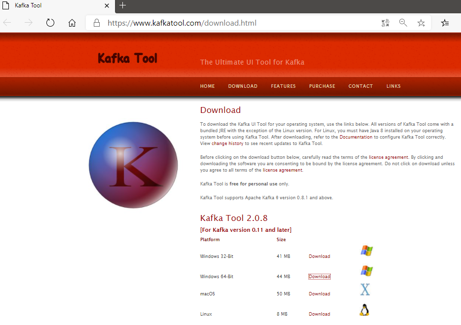
下载地址

http://www.kafkatool.com/download.html

下载界面

不同版本的Kafka对应不同版本的工具,最新的2.0.8版本适合Kafka 0.11和比这更高的版本。

image-20201220144113429

如果是Windows,下载对应的64或者32位的exe文件,一键安装即可。

Kafka Tool 工具使用

1、Kafka 连接配置

1)启动 Kafka Tool

在安装目录下,双击可执行文件 kafkatool.exe,启动 Kafka Tool

img

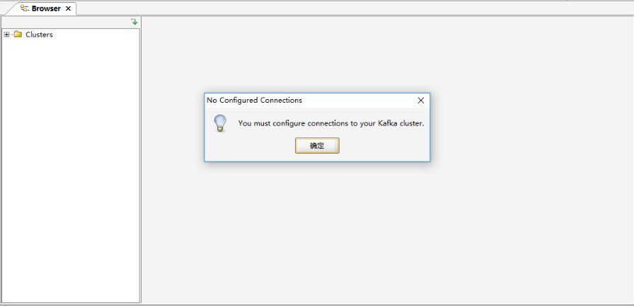
2)配置 Kafka 连接信息

提示配置相应的连接信息

img

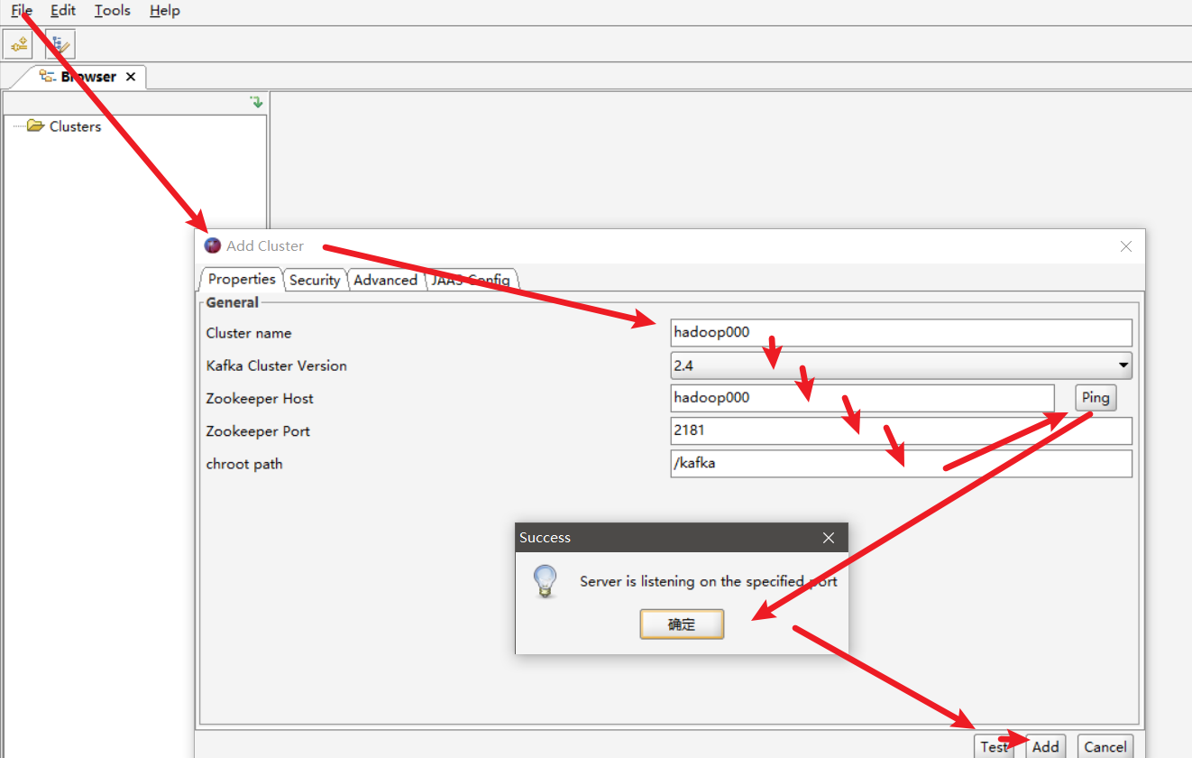
依次填写红框中的信息,点击“Ping” 和 “Test”测试连接情况;测试通过后,点击“Add”进行添加

image-20201220145123007

【注意】这之前需要在 C:\Windows\System32\drivers\etc 下的 hosts 文件中,添加入 kafka 的集群域名

例如,添加如下配置(此处需要根据实际情况配置,配置保存后,需要重启KafkaTools才能读取hosts文件中的内容):

10.10.21.100 hadoop000 
10.10.21.101 hadoop001 
10.10.21.102 hadoop002
10.10.21.103 hadoop003

2、查看 Kafka 数据

1)查看 Kafka 数据

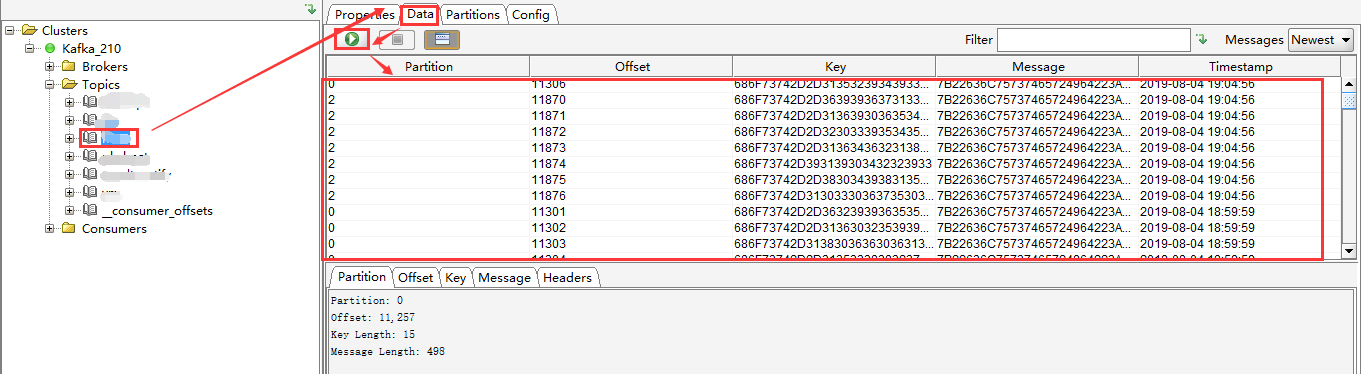
选择一个Topic --> Data,点击查询即可看到数据(但是Key和Message是二进制的,不能直观的看到具体的消息信息,需要设置展示格式)

Messages选择Newest,表示当有新信息来的时候,查看最新的Kafka数据;

结果列表中的每列,通过点击表头,可以按照升序或者降序排序(一般用在时间字段排序,方便查看最新数据)。

img

2)设置 Kafka 数据展示格式

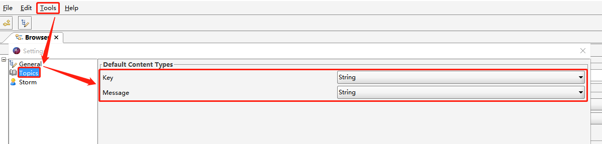
在Tools -->Settings --> Topics,将 Key 和 Message 均设置为String 保存。这样是全局设置,对所有 Topic 均生效。

img

img

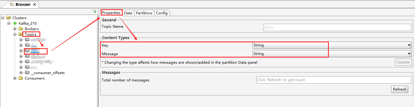
如果只是想单独设置某个 Topic,可以选中某个 Topic,在 Properties --> Content Type 中,将显示格式设置为String,点击 Update --> Refresh 即可生效

img

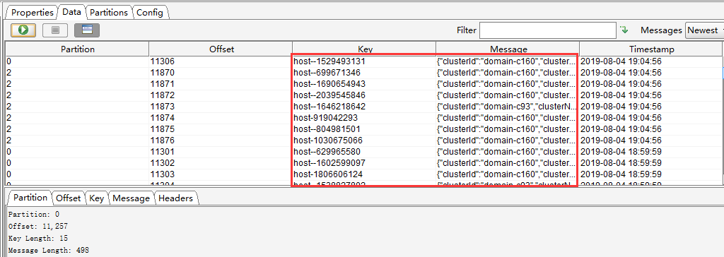
设置后的数据列表如下

img

3)查看具体某一条消息

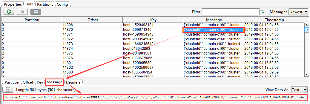
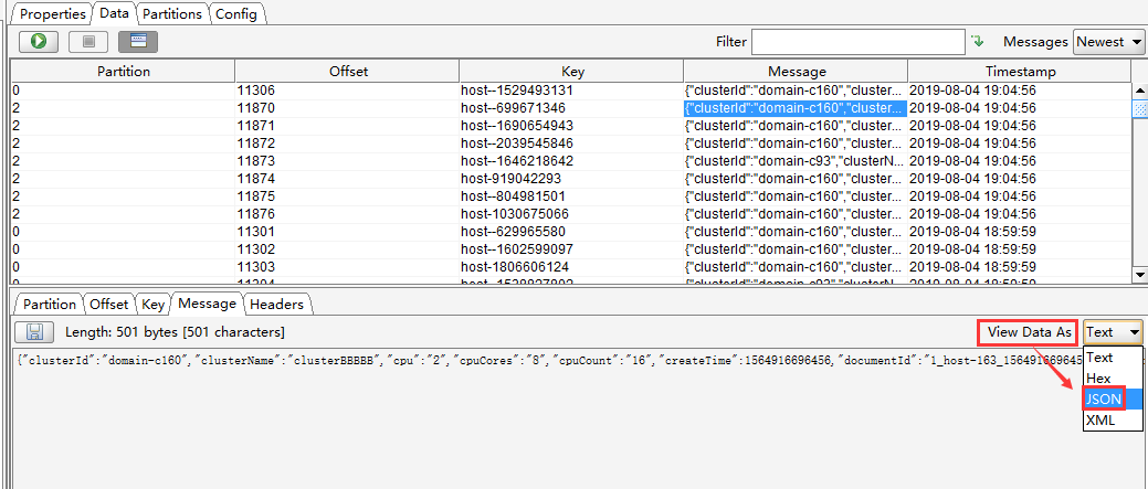
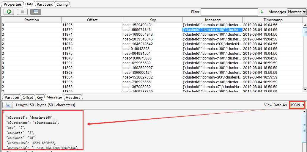
选中某一个message,点击“Message”查看详情,默认是“Text”格式(如果想看到JSON格式,只需要设置下“View Data As”即可)

img

img

“View Data As”设置为 JSON 后,消息信息格式如下

img

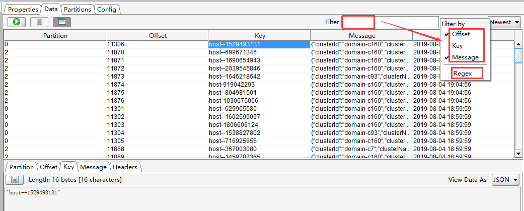
4)过滤查询 Kafka 消息

可以按照Offset(偏移量),Key(消息key),Message(消息主体),Regex(正则表达式)进行单个或者组合查询

img

Views: 276

Kakfa管理操作的相关命令

主题操作

kafka-topics.sh脚本可以用来管理主题.

--topic 指定操作的主题名,除了创建之外都可以使用正则表达式,但是要使用\转义。另外命名不要使用两个下划线开头(__表示系统内建的主题,比如__consumer_offset),主题命名中不要将.和_混用(kafka会将.最终转换成_)。

创建主题

kafka-topics.sh --bootstrap-server hadoop000:9092 --create --topic test-1 --partitions 2 --replication-factor 2

注意: --bootstrap-server 后不要使用localhost, 而是跟上主机名

kafka-topics.sh --bootstrap-server hadoop000:9092 --create --topic test-2 --partitions 2 --replication-factor 2

--zookeeper localhost:2181/kafka 这样的写法从Kafka 2.2版本开始废弃,新版本kafka推荐使用--bootstrap-server替换

其中localhost:2181/kafka 来自于 kafka的server.propertieszookeeper.connect的配置

描述主题

列出所有主题详情

kafka-topics.sh --bootstrap-server hadoop000:9092 --describe

支持正则表达式

 ~]$ kafka-topics.sh --bootstrap-server hadoop000:9092 --describe --topic test-\.\+

修改主题

alter不能修改副本因子。分区数只能增加,不能减少

kafka-topics.sh --bootstrap-server hadoop000:9092 --alter --topic test-1 --partitions 3

删除主题

--delete 只是标记主题为删除状态, 并不会马上删除, 如果你希望立即从zookeeper中删除此主题的信息, 可以在配置文件 server.properties 添加配置 delete.topic.enable=true

kafka-topics.sh --bootstrap-server hadoop000:9092 --delete --topic test-2

列出主题

只列出主题名称, 不带详细信息

kafka-topics.sh --bootstrap-server hadoop000:9092 --list

消费者操作

使用 kafka-consumer-groups.sh 工具,我们可以列出、描述或删除消费者组。消费者组可以被手动删除,也可以在该组最后一次提交的偏移量到期时被自动删除。手动删除仅在组中没有任何活动成员时有效。

列出消费者群组

> bin/kafka-consumer-groups.sh --bootstrap-server hadoop000:9092 --list
test-consumer-group-1
test-consumer-group-2
test-consumer-group-3

如果使用新的消费者客户端,要列出消费者组,可以使用--bootstrap-server和--list选项。因为新的客户端已经删除了--zookeeper选项。

描述消费者群组

> bin/kafka-consumer-groups.sh --bootstrap-server hadoop000:9092 
--describe --group my-group

TOPIC PARTITION CURRENT-OFFSET LOG-END-OFFSET LAG CONSUMER-ID HOST CLIENTID
topic1 0  854144 855809 1665 consumer1-3fc8d6f1-581a-4472-bdf3-3515b4aee8c1 /127.0.0.1 consumer1
topic2 0  460537  803290  342753  consumer1-3fc8d6f1-581a-4472-bdf3-3515b4aee8c1 /127.0.0.1 consumer1 
topic3 2  243655  398812  155157  consumer4-117fe4d3-c6c1-4178-8ee9-eb4a3954bee0 /127.0.0.1 consumer4

删除消费者群组

> bin/kafka-consumer-groups.sh --bootstrap-server localhost:9092 
--delete --group my-group --group my-other-group
Deletion of requested consumer groups('my-group', 'my-other-group') was successful.

当要删除的消费者组不为空时,执行上面命令你将得到以下错误: GroupNotEmptyException

消费偏移量管理

删除偏移量

删除某个主题的某个消费者组的偏移量

> kafka-consumer-groups.sh --bootstrap-server hadoop000:9092 --delete-offsets --group my-group --topic my-topic-1 --topic my-topic-2
TOPIC                          PARTITION       STATUS 
my-topic-1                     0               Successful
my-topic-2                     0               Successful

○当要删除的消费者组不为空时,执行上面命令你将得到以下错误: GroupNotEmptyException

重置偏移量

要重置消费者组的偏移量,可以使用“--reset-offsets”选项。此选项一次只支持一个消费者组。它需要定义以下范围: --all-topic 或 --topic。必须选择一个作用域,除非使用 “--from-file”从文件导入的方式。

> bin/kafka-consumer-groups.sh --bootstrap-server localhost:9092 --reset-offsets --group consumergroup1 --topic topic1 --to-latest
TOPIC                          PARTITION  NEW-OFFSET
topic1                         0 

如果您使用的是旧的高级消费者,也就是消费者组元数据是存储在ZooKeeper中(即配置了offset .storage=ZooKeeper),则需要使用--zooKeeper而不是--bootstrap-server

配置项 描述
–-to-datetime 重置为某个时间点的偏移量.格式: 'YYYY-MM-DDTHH:mm:SS.sss'
--to-earliest : 重置为最早的偏移量
--to-latest : 重置为最近的偏移量
--shift-by : 将当前的偏移量偏移n个单位, n可以为正数也可以是负数
--from-file : 利用CSV文件中的数据重置偏移量
--to-current : R将偏移量重置为当前值
--by-duration : 重置偏移量为从当前时间戳开始的时长, 格式: 'PnDTnHnMnS'
--to-offset : 重置偏移量为指定的值

动态配置修改

从Kafka 1.1.0 开始有了动态配置修改的新特性。动态意味着在修改了Broker的配置后,我们不需要重新启动Broker来使其生效。

这个新特性包含在一个名为kafka-configs.sh的命令行工具脚本中。一旦使用这个工具设置了配置参数,新的更改将永久存储在zookeeper集群中。

覆盖主题默认配置

有许多应用于主题的配置,可以针对单个主题更改这些配置以适应集群中的不同用例。大多数配置都在代理配置中指定了缺省值,除非设置配置覆盖,否则将应用该缺省值。

格式

kafka-configs.sh --bootstrap-server <broker_list> --alter --entity-type topics --entity-name <topic name> --add-config <key>= <value>[,<key>=<value>...]

例子

# 下面的示例将my-topic主题的留存时间设置为1小时,即3600000ms:
$ kafka-configs.sh --bootstrap-server hadoop000:9092 --alter --entity-type topics --entity-name my-topic --add-config retention.ms=3600000

主题的有效可覆盖配置

配置(Key 说明
cleanup.policy 如果设置为compact,则topic中 的消息将被丢弃,仅保留具有给定key的最新消息(日志压缩)。
compression.type broker将消息写入磁盘时使用的压缩类型,可以用gzip、snappy和lz4.
delete.retention.ms 压缩日志墓碑消息的最长存放时间
file.delete.delay.ms 从磁盘中删除此topic的日志端和索引之前需要等待的多长时间
配置(Key 说明
flush.messages 在强制将此topic的消息刷到磁盘之前接收的消息数
flush.ms 在强制将此topic的消息刷到磁盘之前需要的时间,单位是毫秒
index.interval.bytes 日志段索引中的条目之间可以产生多少字节的消息
max.message.bytes 此topic中当个消息的大小
retention.bytes 为topic保留的消息量的总字节数
retention.ms topic中消息保留的最长时间,单位是毫秒

描述覆盖的配置

可以使用命令行工具kafka-configs.sh来检查主题或客户机的特定配置。显示覆盖的配置需要使用--describe选项。例如,一下代码显示名为my-topic的主题的所有覆盖过的配置

> kafka-configs.sh --bootstrap-server <broker_list> --describe --entity-type topics --entity-name my-topic

Configs for topic 'my-topic' are retention.ms=3600000

覆盖客户端默认配置

Kafka客户端(生产者和消费者)唯一可以覆盖的配置是生产者和消费者的配额,即允许具有指定客户端ID的所有客户端在每个broker上每秒生产或者消费的字节数。

格式

> kafka-configs.sh --bootstrap-server <broker_list> --alter --entity-type clients --entity-name <client ID> --add-config <key>=<value>[,<key>=<value>...]

Kafka客户端的有效配置

配置key 描述
producer_bytes_rate The amount of messages, in bytes, that a singe client ID is allowed to produce to a single broker in one second.
consumer_bytes_rate The amount of messages, in bytes, that a single client ID is allowed to consume from a single broker in one second.

如何把Broker中的生产者客户端ID为client_a的配额producer_byte_rate设置成20MB/秒?

> bin/kafka-configs.sh
 --bootstrap-server hadoop000:9092 
 --alter
 --entity-type clients 
 --entity-name client_a
 --add-config 'producer_bytes_rate=20971520'

注意:

  • --add-config 可以同时指定多个配置, 配置之间使用逗号分割

  • 要指定生产者或者消费者的client_id,如果是Java APIs可以为客户端添加配置client.id, 如果是控制台生产者或者消费者可以使用--producer.config--consumer.config进行指定配置文件并且在配置文件中指定client.id.

移除覆盖的配置

可以完全删除动态配置,这将导致集群配置恢复到默认值,要删除配置覆盖,请使用--alter命令以及--delete-config命令。

下面的示例可以删除一个名为my-topic的主题的覆盖后的retention.ms配置, 删除后retention.ms将恢复为默认值:

kafka-configs.sh --bootstrap-server hadoop000:9092 --alter --entity-type topics --entity-name my-topic --delete-config retention.ms

Completed updating config for entity: topic 'my-topic'.

Views: 641